Computing with Oscillators
We developed a PCB to realize the weighted Kuramoto model using coupled electronic oscillators. It is designed for combinatorial optimization and takes the form of an oscillator-based Ising machine (OIM). Interestingly, as the number of oscillators (variables) increases, the number of required cycles (time-to-solution) seems to remain constant. More broadly, these dynamics can be modelled as probabilistic bits (p-bits) for more general learning and optimization tasks. There is a zoo of research to develop p-bit hardware for such tasks due to the power/speed advantages of exploiting a physical process to perform computation. However, these devices remain in academic research largely due to their limited scalability and adoption. They lost the hardware lottery.
The SOTA devices uses fully-digital p-bits implemented on FPGAs or ASICs using modern process nodes. While the OIM is not necessarily the best architecture, it can be realized with a basic breadboard and scaled on a low-cost PCB as an experimental testbed. Our PCB contains 8 LC oscillators (top board) connected through a programmable resistive network (bottom board).
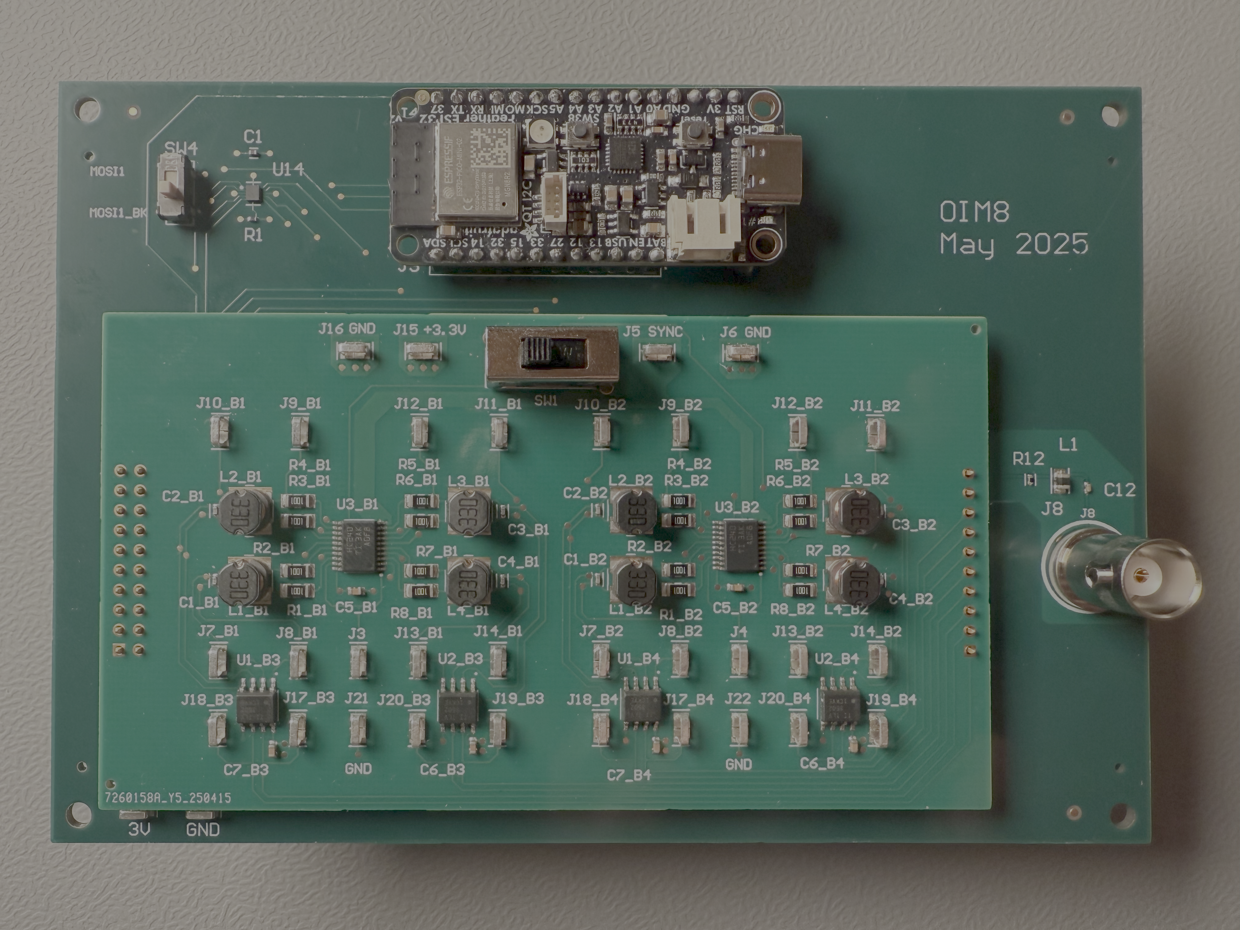
The system is a fully-connected graph, where each node is a LC oscillator, and each edge is a tunable resistor. It can therefore be used to solve an 8-variable binary optimization problem.
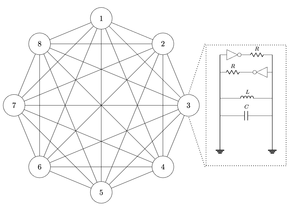
The theory of OIMs maps the phase of each oscillator $\theta_i$ to a binary variable $x_{i}$. The ESP32 controls resistive couplings (8-bit digital potentiometers) between each oscillator to encode the matrix $\mathbf{J}$ that defines the problem. The oscillators will then stabilize to phase configurations that minimize \begin{equation} H(x) = x^{T}\mathbf{J}x \end{equation} This quadratic optimization is generally NP-Hard and represents a board class of problems. The weighted Kuramoto model admits an equivalent Lyapunov function, meaning the natural phase dynamics can be exploited to minimize $(1)$. In fact, these dynamics actually implement continuous-time Lagrange multiplier optimization. However, in our case, we must ensure the phases settle to discrete binary (0 or $\pi$) values instead of continuous ones. To do this, an external perturbation signal at twice the oscillation frequency is used to create bi-stable modes, a technique known as subharmonic injection locking. The amplitude can be varied over time, which effectively performs annealing to gradually enforce bi-stability. This is required because not all stable phase configurations represent the global minimum of $(1)$.
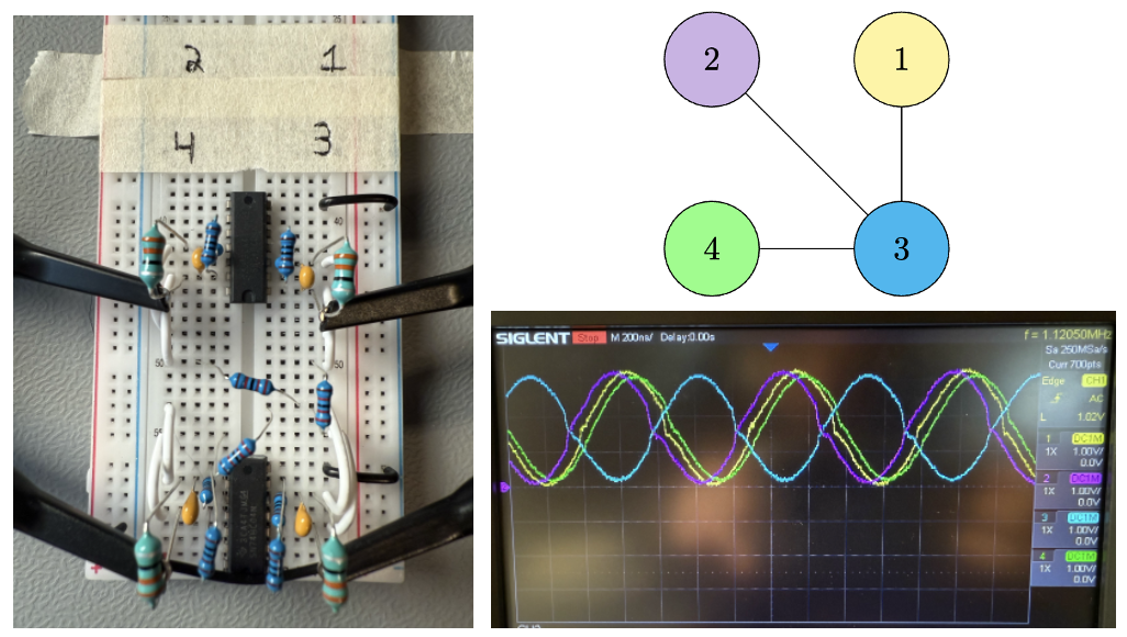
As mentioned, this principle can be demonstrated with a simple breadboard experiment. In this example, 10K ohm resistors connect the variable $x_3$ (blue) to $x_1$ (yellow), $x_2$ (purple), and $x_4$ (green) which themselves share no connections. No injection locking is used for this small experiment. Probes measure the voltage waveform at the inductor at each oscillator. The oscilloscope shows the set of variables $\{x_1, x_2, x_4\}$ are mis-aligned with $\{x_3\}$, which indicates the optimal solution $x^{*} = [1 1 0 1]$ or equivalently $x^{*}=[0 0 1 0]$. In context of the MaxCut problem, this corresponds to “cutting all the resistors” which is the optimal partition for this graph. Although the solution is trivial, it demonstrates how the oscillators can perform the computation “for free”.
This analog approach can be vastly more power-efficient than GPUs or TPUs for combinatorial optimization. Of course, developing a scalable (analog) oscillator network with programmable couplings is a key challenge. In practice, operations research uses a range of deterministic and randomized methods like simulated annealing or Monte Carlo that can cost about 20 nJ per trial bitflip. FPGAs and ASICs can achieve 2-5 orders of magnitude even less energy per bitflip. The energy/bitflip metric allows a basic comparison between different technologies but does not capture other important measures like overall time-to-solution. Nonetheless, it highlights potential alternatives to classical solvers.
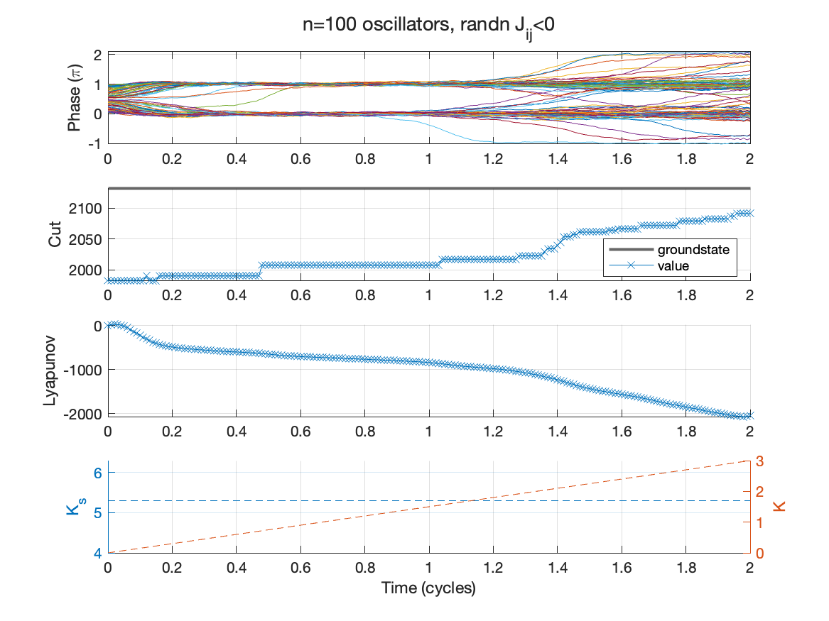
The figure below shows a SDE simulation of the weighted Kuramoto network to solve a 100-variable MaxCut problem. The phase of each oscillator closely aligns to an integer multiple of $\pi$ due to the injection locking (subplot 1). The annealing schedule (subplot 4) ramps an overall gain $K$ and keeps the synchronization gain $K_{s}$ fixed using empirically chosen values. The network almost reaches an optimal phase alignment corresponding to the best cut or groundstate (subplot 2). The Lyapunov function is gradually minimized (subplot 3) even when none of the phases change. This is evident around 0.8 cycles. Note these oscillators generally don’t undergo many phase transitions (bitflips), yet they reliably move the system towards the optimal alignment.
There is lots of theoretical bifurcation and stability research on variants of the Kuramoto model, but applications to combinatorial optimization are limited. In general, the optimal annealing schedule can be understood as optimal control of a non-equilibrium system. This remains an open problem. However, recent work shows that thermodynamically optimal paths minimize entropy production. Our work is grounded in statistical mechanics to show how multi-dimensional control can improve performance on constrained problems and give suitable annealing schedules, rather than the heuristics commonly used in practice. The PCB illustrated here is a proof-of-concept towards this goal.